scipy: Unexpectedly poor results when distribution fitting with `weibull_min` and `exponweib`

A good start value is crucial for the ML method to find a good solution, especially if many parameters are to be estimated. So if weibul_min had a better _fitstart function like this:

>>> import numpy as np

>>> def _fitstart(data): 
...      """Reference: Cohen & Whittle, (1988) "Parameter Estimation in Reliability
...           and Life Span Models", p. 25 ff, Marcel Dekker
...      """
...      loc = data.min() - 0.01  #*np.std(data)  # alternatively subtract 0.01*stdev
...      chat = 1. / (6 ** (1 / 2) / np.pi * np.std(np.log(data - loc)))
...      scale = np.mean((data - loc) ** chat) ** (1. / chat)
...      return chat, loc, scale

it would solve many situations of unexpectedly poor results when fitting the weibul_min distribution so the user wouldn’t have to fiddle to finetune the fitting. Below I have compared the start values obtained from the default stats.weibull_min._fitstart method the method above. And it is clear that that the bad startvalue for the parameters are the cause of this poor fit:

>>> from scipy import stats

>>> x = [4836.6, 823.6, 3131.7, 1343.4, 709.7, 610.6, 
...     3034.2, 1973, 7358.5, 265, 4590.5, 5440.4, 4613.7, 4763.1, 
...     115.3, 5385.1, 6398.1, 8444.6, 2397.1, 3259.7, 307.5, 4607.4, 
...     6523.7, 600.3, 2813.5, 6119.8, 6438.8, 2799.1, 2849.8, 5309.6, 
...     3182.4, 705.5, 5673.3, 2939.9, 2631.8, 5002.1, 1967.3, 2810.4,
...     2948, 6904.8]

>>> data = np.asarray(x)
>>> _fitstart(data)
...  (0.5899119992937546, 115.28999999999999, 3060.830920639086)
>>> stats.weibull_min._fitstart(data)
...  (1.0, -717.6300000000002, 1)

>>> chat, loc, scale =_fitstart(data)
>>> stats.weibull_min.fit(x, chat, loc=loc, scale=scale)
(1.7760067130728838, -322.09255199577206, 4355.262678526975)

Kidding aside, if “loc = x” had a little more influence that would be a good thing.

You mean if providing the guess loc=x was a stronger hint, it would be preferable? I see. Even if you provide loc=0, SciPy finds the crazy solution. But perhaps that is because there is not a local minimum of the objective function for it to settle into that is near loc=0.

I’m not sure if we can bake what you’re looking for into the fit method. Maximum Likelihood Estimation is a specific way of fitting a distribution to data, and I think SciPy is doing a reasonable job of that here. You may want to define your own objective function that includes a mathematical description of sanity : )

I’m only partially joking. It’s really not too tough to fit using minimize directly. Assuming you’ve already run the code above:

from scipy.optimize import minimize
def ll(params, data):
    # negative of log likelihood function as we're minimizing
    return -np.sum(np.log(weibull_min.pdf(x, *params)))

res = minimize(ll, (6.4, 0, 21.6), args=(x,))
c3, u3, s3 = res.x
pdf3 = weibull_min.pdf(q, c3, loc=u3, scale=s3)

plt.plot(q, pdf, '-', q, pdf2, '--', q, pdf3, '-')
plt.hist(x, density=True, alpha=0.5)
plt.title(f"weibull_min fits")
plt.legend((f"pdf(c={c:.2}, loc={u:.2}, scale={s:.2})",
            f"pdf(c={c2:.3}, loc={u2}, scale={s2:.3})",
            f"pdf(c={c3:.3}, loc={u3:.2}, scale={s3:.3})",
            "observations"))

produces

This is not much better, but the point is that now you can change the objective function or add constraints to get something closer to what you’re looking for. (It’s just not maximum likelihood estimation anymore.)

(Note: this comment restates and adds some details to some of what @josef-pkt has already said.)

The problem that fit attempts to solve is to find the maximum of the likelihood function. For the weibull_min distribution with three parameters, this is

L(x, c, a, s) = prod( (c/s) * ((x[i] - a)/s)**(c - 1) * exp(-((x[i] - a)/s)**c )

where c > 0 is the shape parameter, and for brevity, a is the location and s > 0 is the scale.

Now suppose the x values are sorted in increasing order, so x[0] is the minimum of all the x values. Also suppose c is any value such that 0 < c < 1, so c - 1 < 0. Then, as a -> x[0] from below, the term ((x[0] - a)/s)**(c - 1) blows up, while the other terms in the product approach well-defined limits. So by moving the location parameter closer and closer to x[0], we can make the likelihood function as large as we like. We might say, then, that we should pick the minimum of x as the estimate of the location parameter. But note that we have done that without specifying c or s, other than 0 < c < 1 and s > 0. So there is not a unique, well-defined solution in this case.

The code in SciPy implements fit by minimizing the negative of the log of the likelihood, and it is attempting to do this using a solver that expects the numerical problem to be well-behaved. But the negative log-likelihood has the same problem as the likelihood: by making the location approach the minimum from below, the negative log-likelihood goes off to negative infinity, for any values of 0 < c < 1 and s > 0.

So we can’t really expect useful results from weibull_min.fit when the location parameter is not fixed. (The same is true for weibull_max, and for some other distributions.) Perhaps the safest choice (already mentioned above) is to simply not allow it, by raising an exception if the location is not fixed.

It looks like the fit function is doing what it is supposed to do here, it’s just that the default optimizer is not doing a great job. It would be nice to improve it, but it’s not a simple fix.

One thing you could try, @nayefahmad, is to use a different optimizer. For instance, I got pretty good results with differential_evolution here.

bounds = [(0, 5), (0, 5000), (0, 5000)]
def optimizer(func, x0, args, disp):
    res = differential_evolution(func, bounds, args)
    return res.x

shape, loc, scale = stats.weibull_min.fit(x, optimizer=optimizer, method="MLE")
print(shape, loc, scale)

It’s stochastic, but I’ve gotten as good as: 1.5017832616353088 0.0 3912.5900933784724

Although I disagree with the rationale above* for why we can’t expect good results when loc is not defined, the conclusion is correct.

As in this post about Nakagami, a plot of the NLLF shows the real reason why either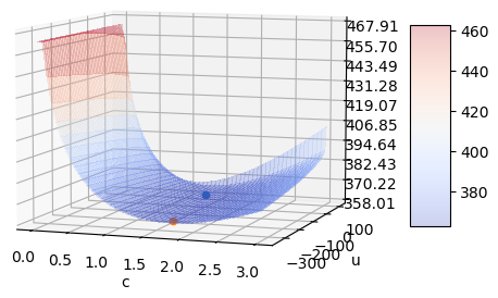 loc or c needs to be fixed - the distribution is nearly over-parameterized for c sufficiently greater than 1. Here is the NLLF as a function of c and loc with scale set at its analytical optimum (for the given values of the other parameters).

The blue point is the one fit gives you when floc=0. The orange point is what I got above when I solved the first-order necessary conditions.

weibull_min.nnlf((1.501782497874548, 0, 3912.846255032002), x)  # Bluie, 363.2264489714531
weibull_min.nnlf((1.7760069940171093, -322.09251325529544, 4355.263216573265), x)  # Orange, 363.00129740378594

They’re in a long valley where the NLLF barely changes for large changes in the parameters. The orange point is ever so slightly better in the MLE sense.

(I imagine this is typical for c sufficiently greater than 1. I’ll check some of the other cases above after posting this.)

To close this issue, I’d suggest the following:

• Mention that for best fit results, users should fix loc - probably at 0.
• Override the default fit method when loc or c are fixed. In either case, we have an analytical solution for the scale, and we can solve the first-order necessary condition for the remaining parameter with root_scalar.
• Override _fitstart similar to how we did in Nakagami, but instead of using loc = np.min(data), make it a little less than that. we can find an approximation for c in the literature, or we can guess using the relationship between the parameters and mean/variance (method of moments, basically. Update: @pbrod gave a suggestion above.
• Unlike Nakagami, the default fit method is frequently having trouble with all parameters free, so if a _fitstart override doesn’t help, we should try to override the default fit method even when loc and c aren’t fixed. I think that using the analytical solution for scale inside the objective function will help, or we can use the analytical solution for scale and try to solve the first-order necessary conditions as above.

---

* For sufficiently small c, the best fit for loc is np.min(data), whether the LLF is blowing up or not. There is still some sense in which we can maximize the LLF even if we can make it as large as we please. The same thing happens for several distributions; another example of this discussion is in gh-11782, so I won’t repeat it here.

---

Update: @jkmccaughey’s example above has an even more extreme valley.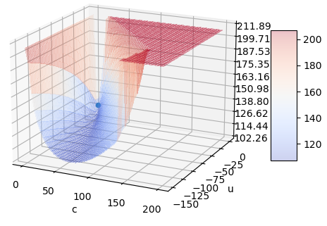

As discussed above, a slightly better MLE than (6.438181305640674, 0, 21.607076911881855) is (34780967.41119945, -91088178.5479899, 91088200.47560324)!

@swallan Maybe this after Nakagami.

Algorithms are weird!

I wrote a little code to investigate:

import numpy as np
from scipy.stats import weibull_min
import matplotlib.pyplot as plt

x = [2.03,8.51,11.14,13.79,16.11,17.32,18.15,18.67,19.07,19.43,19.70,19.99,20.19,20.40,20.59,20.76,20.93,21.08,21.24,21.37,21.50,21.63,21.75,21.87,21.99,22.09,22.19,22.31,22.41,22.50,22.62,22.75,22.87,22.99,23.13,23.28,23.45,23.67,23.91,24.29,26.42]
c, u, s = weibull_min.fit(x)
c2, u2, s2 = weibull_min.fit(x, floc=0)

# print(a, u, s)
q = np.arange(0, 30, 0.1)

pdf = weibull_min.pdf(q, c, loc=u, scale=s)

pdf2 = weibull_min.pdf(q, c2, loc=u2, scale=s2)

plt.plot(q, pdf, '-', q, pdf2, '--')
plt.hist(x, density=True, alpha=0.5)

plt.title(f"weibull_min fits")
plt.legend((f"pdf(c={c:.2}, loc={u:.2}, scale={s:.2})",
            f"pdf(c={c2:.3}, loc={u2}, scale={s2:.3})",
            "observations"))

ll = np.sum(np.log(weibull_min.pdf(x, c, loc=u, scale=s)))
ll2 = np.sum(np.log(weibull_min.pdf(x, c2, loc=u2, scale=s2)))
print(ll, ll2)

Qualitatively, both fit the data pretty well: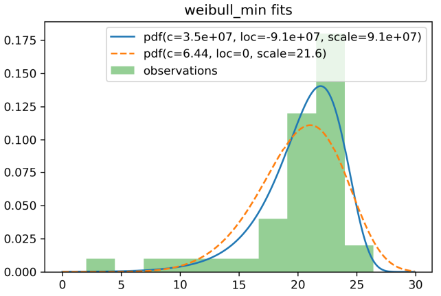

and it turns out that the fit with ridiculous looking numbers (the first one) has a bit higher (less negative) log-likelihood:

-106.79743088776479 -116.75415467840313

Am I doing something incorrectly with Weibull_min?

It doesn’t sound like you’re doing something incorrectly. You’ve found that for a good estimate, sometimes it helps to fix one of the values. We’re working on improving the starting guesses and adding analytical fits where possible, but if those things are not implemented, fit just tries to solve an optimization problem numerically. It doesn’t pay attention to whether the values of shape, loc, and scale look reasonable; it just cares about optimizing the objective function (which is the LL function w/ a penalty for data beyond the support of the distribution), and it’s not guaranteed to find the global optimum. weibull_min may be one of those distributions for which the objective function is relatively flat w.r.t. certain changes of parameters, so providing a good guess or fixing one parameter can go a long way to improving how reasonable the fit parameters are!

@nayefahmad You probably don’t need this anymore, but I also get good results by solving the first-order conditions. There is an explicit formula for the scale, and the shape and location can be determined using root.

import numpy as np
from scipy import stats
from scipy.optimize import root
from scipy.stats import weibull_min
import matplotlib.pyplot as plt

np.random.seed(0)

x = [4836.6, 823.6, 3131.7, 1343.4, 709.7, 610.6,
     3034.2, 1973, 7358.5, 265, 4590.5, 5440.4, 4613.7, 4763.1,
     115.3, 5385.1, 6398.1, 8444.6, 2397.1, 3259.7, 307.5, 4607.4,
     6523.7, 600.3, 2813.5, 6119.8, 6438.8, 2799.1, 2849.8, 5309.6,
     3182.4, 705.5, 5673.3, 2939.9, 2631.8, 5002.1, 1967.3, 2810.4,
     2948, 6904.8]
x = np.array(x)


def ll(dist, data, *args):
    # log-likelihood function
    return np.log(dist(*args).pdf(data)).sum()


def get_s(c, u, x):
    # analytical solution for scale, given shape and location
    N = len(x)
    return (1/N * ((x-u)**c).sum())**(1/c)


def f(z, x):
    N = len(x)
    c, u = z
    s = get_s(c, u, x)
    # partial of LL w.r.t. shape
    dldc = c + N/((1 - ((x-u)/s)**c) * np.log((x-u)/s)).sum()
    # partial of LL w.r.t. location
    dldu = ((-c * ((x-u)/s)**c + c - 1)/(u - x)).sum()
    return [dldc, dldu]


res = root(f, np.random.rand(2), args=(x,))
c, u = res.x
s = get_s(c, u, x)

print(fr"c = {c}, u = {u}, s = {s}")
d = 0.0001
print(f"Diffs of the LL w.r.t. d = {d} change in the parameters are:")
diff = [ll(weibull_min, x, c, u, s) - ll(weibull_min, x, c, u, s+d),
        ll(weibull_min, x, c, u, s) - ll(weibull_min, x, c, u, s-d),
        ll(weibull_min, x, c, u, s) - ll(weibull_min, x, c, u+d, s),
        ll(weibull_min, x, c, u, s) - ll(weibull_min, x, c, u-d, s),
        ll(weibull_min, x, c, u, s) - ll(weibull_min, x, c+d, u, s),
        ll(weibull_min, x, c, u, s) - ll(weibull_min, x, c-d, u, s)]
print(diff)

fig, ax = plt.subplots(1, 1)
xpdf = np.linspace(weibull_min.ppf(0.01, c, u, s),
                   weibull_min.ppf(0.99, c, u, s), 100)
ax.plot(xpdf, weibull_min.pdf(xpdf, c, u, s),
       'r-', lw=5, alpha=0.6, label='weibull_min pdf')
ax.hist(x, density=True, histtype='stepfilled', alpha=0.2)
ax.legend(loc='best', frameon=False)
plt.show()

outputs:

c = 1.7760067996300921, u = -322.0926637141707, s = 4355.262877063057
Diffs of the LL w.r.t. d = 0.0001 change in the parameters are:
[5.684341886080802e-14, 5.684341886080802e-14, 1.1368683772161603e-13, 1.1368683772161603e-13, 1.0197209121542983e-07, 1.0197669553235755e-07]

Hi everyone I work in the sector of offshore energy and I analyse data describing meteorological conditions (such as wind speed, wave height, tidal stream speed, …) I also had problems by fitting the weibull_min distribution to data. Through empirically trying different options, I found out that by setting: location parameter first guess = (mean of the data) * 0.3   scale parameter first guess = mean of the data     I usually obtain reasonably good fitting. Of course the correct solution is to improve the fitting algorithm for this distribution but, in the meantime, maybe the first guess I’m utilising could be useful for other types of data as well.

OK. There is already an issue gh-11751 that mentions improving the optimizer. I think I’ll combine them. If you’d summarize your takeaways on stackoverflow, I’d appreciate it!

Sorry, what’s the difference between setting loc=0 and setting floc=0?

loc=0 is a guess for the optimizer to start with. It iteratively improves upon the guess. floc fixes the value of loc to 0.

Actually, @nayefahmad , the parameter optimization problem is small enough that brute works quite well.

bounds = [(0, 5), (0, 5000), (0, 5000)]
def optimizer(func, x0, args, disp):
    return brute(func, bounds, args)

shape, loc, scale = stats.weibull_min.fit(x, optimizer=optimizer, method="MLE")
print(shape, loc, scale)

gives

1.7760066970837123 -322.09250000052634 4355.262707518204

If the objective function in SciPy is correct, then this is a better fit than the one R gave.

Still, I think @nayefahmad has a point - I’ve confirmed that the minimizer is not converging to a great local minimum. I’m going to look into using the other optimizers to see if they work better on this one.

Hi @nayefahmad, I’m working on improving the fit functionality these days (gh-11695, gh-11782), so thanks for submitting this test case. I’ll look into this soon.